Contact Us : 800.874.5346 International: +1 352.375.0772


Excel operates on cell references – that is how the cells in the worksheets refer to each other. Cell references are the basis of all Excel operations. An understanding of cell references is thus critical for Excel users.
Excel does not directly interpret the data in the cells, but rather the positions (i.e., cell names) of the cells containing the data.
For example, consider the following dataset (you may paste the bordered section in Excel):
| A | B | C | D | E | |
| 1 | Data | 2017 | 2018 | 2019 | 2020 |
| 2 | Sales | 2,000,000 | 3,000,000 | 4,000,000 | 5,000,000 |
| 3 | Gross Profit | 1,400,000 | 2,100,000 | 2,800,000 | 3,500,000 |
| 4 | Net Profit | 400,000 | 600,000 | 800,000 | 1,000,000 |
To find the total sales from 2017 to 2020 and store the total sales in cell F2, we need to add up the contents in cells B2 through E2 in cell F2. We can type in cell F2 the formula = B2 + C2 + D2 + E2 (instead of typing = 2000000 + 3000000 + 4000000 + 5000000 in cell F2) to get the total sales amount of $14 million.
Using the formula is more efficient, provides less room for error, and yields the same result as manually typing the numbers. (For the simple rules of Excel calculations, see Excel Calculation Rules.)
Because the calculation is based on the cell names (i.e., B2, C2, D2, and E2), the result will immediately change to reflect any change in the content of the cell. For example, if we change the content in cell D2 to 5,000,000, the result in cell F2 will immediately change to $15 million.
It is the feature of relative reference that makes it so easy and powerful to do calculations in Excel.
Under relative references, Excel automatically changes the relative positions of the cells in the formula when we copy and paste the formula.
We use the formula = B2 + C2 + D2 + E2 in cell F2 to compute the total sales. If we want to calculate the total gross profit and total net profit for the years, instead of typing the formulas = B3 + C3 + D3 +E3 and =B4 + C4 + D4 + E4, we can copy the formula in cell F2 and paste it in cells F3 and F4.
In this way, the formula from cell F2 is automatically updated to reflect the relative positions: rows 3 and 4 rather than row 2. Similarly, when pasted to cell F4, the formula will automatically change to = B4 + C4 + D4 + E4.
The following methods can be used to paste the formula:
Consider the following example:
| A | B | C | D | E | |
| 1 | Data | 2017 | 2018 | 2019 | 2020 |
| 2 | Sales | 2,000,000 | 3,000,000 | 5,000,000 | 5,000,000 |
| 3 | Gross Profit | 1,400,000 | 2,100,000 | 2,800,000 | 3,500,000 |
| 4 | Net Profit | 400,000 | 600,000 | 800,000 | 1,000,000 |
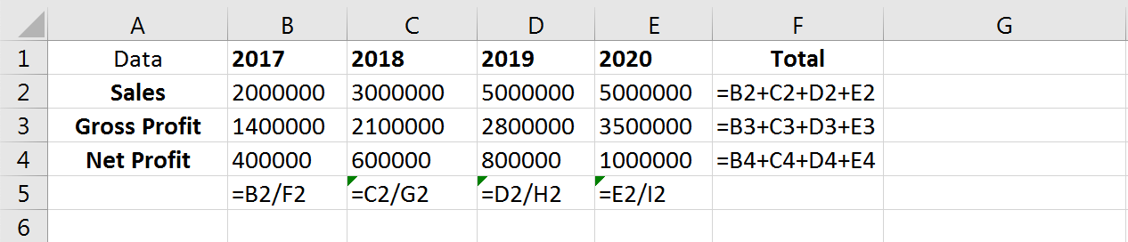
Given that the total sales from 2017 to 2020 is $15 million (stored in cell F2), what is each year’s percentage of total sales?
To find the percentage for 2017, we type the formula = B2/F2 in cell B5. However, when we try to apply (copy and paste) the formula in cell B5 to cells C5 through E5, the “#DIV/0!” error is shown.
When we look at the formulas in the cells, we can see that both the reference to the sales in each year and the reference to the total sale change. There is no content in cells G2 through I2. Thus, we are asking Excel to divide a number by zero. That’s why the “#DIV/0!” error is prompted.
Since we want to divide the sales in each year by cell F2, we should “lock” that cell so that it does not change when we copy and paste the formulas. To “lock” the cell references in B2, we need to use an absolute reference.
Here are two ways to set an absolute reference:
Thus, when we calculate the percentage in 2017 in cell B5, we type the formula = B2/$F$2. When we apply the formula in cell B5 to cells C5 through E5, only the references to the sales in each year (i.e., C2 through E2) will be changed.

Mixed references are combinations of relative reference and absolute reference. Part of the reference is allowed to change and part of it is “locked.” Here are some examples:
| Mixed Reference | Meaning |
|---|---|
| = $B2 | The column is “locked” |
| = B$2 | The row is “locked” |
| = B2: $F$2 | The last cell in the range is “locked” |
| = $B2 : F$2 | The column of the first cell and the row of the last cell in the range are “locked” |
Mixed references are used in more complicated worksheets to improve efficiency and reduce manual input errors.
At Gleim, we know learning data analytics is vital for future accounting professionals. That is why we are offering these series of data analytics blogs and continually updating all of our CPA, CMA, and CIA Review materials with the necessary information you need to pass your exams.
We’ll continue our weekly blog series. Check back regularly for exam news and study tips!
Excel Lessons
Excel Basics
Excel Shortcuts
Excel Calculation Rules
Cell References
Excel Functions
Function Basics
Working with Numbers
Working with Datetime Data
Working with Text Data
Logical Testing
Summarizing Data
Filtering and Sorting
Lookup Functions
Tables
Pivot Tables
Python Lessons
Python Basics
Conditional Statements
Loops
Functions and Modules
Numerical Python (NumPy)
Pandas Basics
Pandas Data Capture and Cleansing
Merging and Grouping
Manipulating Text and Datetime Data
Visualization
Web Scraping
Errors and Exceptions