Contact Us : 800.874.5346 International: +1 352.375.0772


In Excel, a range of cells can be converted to Excel tables to ease data management and analyses. Excel tables provide useful features, including scalable dynamic ranges, more intuitive formulas, and slicers. This blog provides an overview of Excel tables.
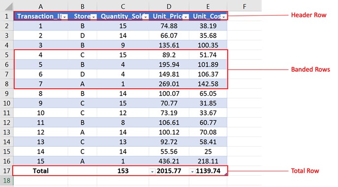
Assume the following dataset [you may paste it to Excel]:
| A | B | C | D | E | |
|---|---|---|---|---|---|
| 1 | Transaction_ID | Store | Quantity_Sold | Unit_Price | Unit_Cost |
| 2 | 1 | B | 15 | 74.88 | 38.19 |
| 3 | 2 | D | 14 | 66.07 | 35.68 |
| 4 | 3 | B | 9 | 135.61 | 100.35 |
| 5 | 4 | C | 15 | 89.2 | 51.74 |
| 6 | 5 | B | 4 | 195.94 | 101.89 |
| 7 | 6 | D | 4 | 149.81 | 106.37 |
| 8 | 7 | A | 1 | 269.01 | 142.58 |
| 9 | 8 | B | 14 | 100.07 | 65.06 |
| 10 | 9 | C | 15 | 70.77 | 31.85 |
| 11 | 10 | C | 12 | 73.19 | 33.67 |
| 12 | 11 | B | 8 | 106.61 | 60.77 |
| 13 | 12 | A | 14 | 100.12 | 70.08 |
| 14 | 13 | C | 13 | 92.72 | 58.41 |
| 15 | 14 | C | 14 | 55.56 | 25 |
| 16 | 15 | A | 1 | 43621 | 218.11 |
To create an Excel table, follow the steps below:
1. Make sure the dataset has headers for each column.
2. Select any datum (cell) in the dataset.
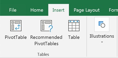
3. On the ribbons, select Insert > Tables [Shortcut key: Ctrl + T].
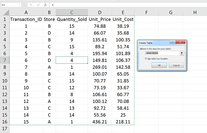
4. Make sure the data range for the table is correct.
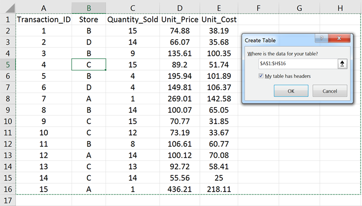
5. Make sure the “My table has headers” box is checked.
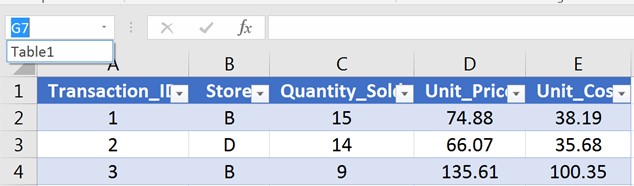
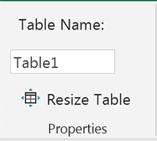
Names of Excel tables are displayed in the name box. By default, they are named Table 1, Table 2, etc. To navigate to the table, select the table name in the name box.
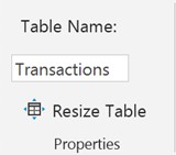
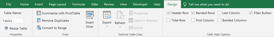
To rename a table, go to Design > Properties > Table Name and change the name.

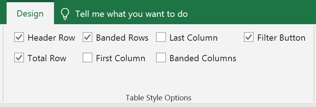
Under the ribbons, select Design > Table Style Options, the different elements of Excel tables can be enabled.
Fields:
Each column in an Excel table is a field. Checking the boxes for “First Column” or “Last Column” makes the two respective fields bold.
Header row:
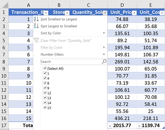
The header row is embedded with Excel Auto Filters to allow users to quickly filter and sort.
Banded Rows/Columns:
Rows (columns) are marked by alternate bandings to help distinguish the rows (columns).
Total Row:
The Total Row contains drop-down lists for each field of the table.
The drop-down list
1. Scalable dynamic range
When columns (rows) are added to, or deleted from, an Excel table, the table automatically expands or contracts to accommodate the change.
To add a column (row), type in the data in the first cell of the new column (row).
To delete a column (row), select the column (row), right click, and select “Delete”.
2. Scalable dynamic range
Cell ranges use explicit cell references (e.g., A1, B10, C3:D9) to refer to individual cells or ranges; Excel tables use structured references to refer to the data. [See “Structured References” ]
Example:

Formula in cell F2 using cell references and structured references:
| Cell references | Structured references |
|---|---|
| = C2 * D2 | =[@[Quantity_Sold]]*[@[Unit_Price]] |
Because structured references use the field names rather than the cell names, formulas under structured references are more intuitive and human-readable.
3. Auto-filled formulas
When a formula is entered into a column (any cell), the formula is automatically applied to the whole column.
4. Slicers
Slicers are an easier way to filter the data compared to the Excel Auto Filter. To use a slicer, follow the steps below:
1. Select any cell in the table.
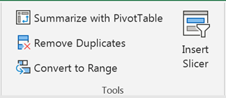
2. Under the ribbons, select Design > Tools > Insert Slicer.
3. Choose the field to be sliced.

4. Click the option sin the slicer to filter the data.
5. Easy rearrangement
To rearrange the columns (rows) of an Excel table, select the whole column (row) in the table (including the Total Row) and drag and drop the column (row) to the desired location in the table. The column (row) will be inserted to the desired location and other columns (rows) will be shifted accordingly.
6. Frozen panel view
When we scroll down an Excel table and the header row is off the screen, the field’s names replace the column indices of the spreadsheet (freezing the header row at the top), thereby keeping the field names visible.
What are structured references
When we create an Excel table, Excel automatically assigns names to the table and its fields. When referring to the data in the table, instead of the cell references, the combination of the table and field name should be used. Such combination is called a structured reference.
Using structured references inside Excel tables
Assume the following Excel table:

Example 1: Using structured reference by clicking and typing.

Example 2: Using structured reference by typing and selecting.
Using structured references outside Excel tables
Outside Excel tables, the structured reference of a data field must comprise both the name of the table and the field name.
Assume an Excel table as the following:
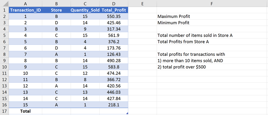
Example 1: Cell references vs. Structured references
Using cell references, the formulas to find the maximum and minimum total profits are =max(D2:D16) and =min(D2:D16).
Using structured references, the formulas to find the maximum and minimum total profits are =max(Table1[Total_Profit]) and =min(Table1[Total_Profit]).
Example 2: Conditional summary
With cell references, the formula =sumif(B2:B16, “=A”, C2:C16) is used to calculate the total items sold in Store A. With structured references, the formula to calculate the total items sold in Store A is =sumif(Table1[Store], “=A”, Table1[Quantity_Sold]).
Structured references are less error-prone when performing logical testing. Table1[Store] = “A” is more intuitive than B2:B16 = “A”.
Example 3: Easing formula adjustment
Using cell references, the formula =sumifs(D2:D16, C2:C16, “>10”, D2:D16, “>500”) finds the total profits for transactions with more than 10 items sold and with profits over $500.
Using structured references, the formula is =sumifs(Table1[Total_Profit], Table1[Quantity_Sold], “>10”, Table1[Total_Profit], “>500”).
When the criteria change and we are calculating the total profits for transactions with more than 8 items sold and with profits over $400, the formula written in cell references does not clearly show the different pairs of criteria range and criteria, whereas the formula written in structured references shows a more human-readable match of the pairs.
To uncreate an Excel table, follow the steps below:
At Gleim, we know learning data analytics is vital for future accounting professionals. That is why we are offering this series of data analytics blogs and continually updating all of our review materials for CPA, CMA, and CIA with the necessary information you need to pass your exams!
We’ll continue our weekly blog series. Check back regularly for all exam news and study tips!
Python Lessons
Python Basics
Conditional Statements
Loops
Functions and Modules
Numerical Python (NumPy)
Pandas Basics
Pandas Data Capture and Cleansing
Merging and Grouping
Manipulating Text and Datetime Data
Visualization
Web Scraping
Errors and Exceptions