Excel Functions: Lookup Functions

Lookup functions are among the most frequently used functions in Excel. For example, the vlookup function is the third most used function (after the sum and average function). Lookup functions look up  a specified element  in a range and return the corresponding information. This blog introduces the basics and some advanced applications of the lookup function.

Single-criterion lookup

vlookup function

The vlookup (vertical lookup) function looks up the value in a range by rows (downwards) and then returns the corresponding information in the same row (rightwards).

Below is an example of how the vlookup function works.

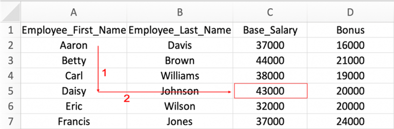
Assume the following dataset about the payrolls of a company:

To look up the base salary of Daisy, the vlookup function looks downwards along the first column until the text “Daisy” (row 5) is found. It then looks rightwards across the columns to find and return the value in the “Base_Salary” column.

The vlookup function has the following syntax:

Example 1: Basic applications

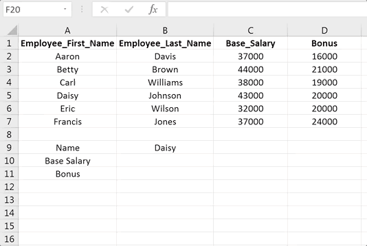
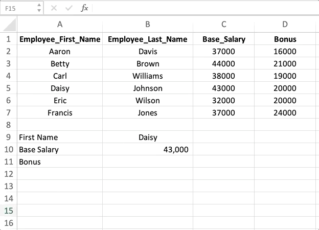
Assume the following dataset [you may paste it to Excel]:

Cell B9 contains the name of the employee to be looked up, and cells B10 and B11 are for displaying the base salary and bonus of the employee.

In cell B10, the formula = vlookup(B9, A1:D7, 3, FALSE) returns the base salary of the employee whose name is specified in cell B9. Here is the process performed:

1. What is the lookup key?
   The value in cell B9 (i.e., Daisy).
2. Where to look up?
   The range A1 through D7.
3. What to look up?
   The base salary of the employee, which is in the 3^rd column of the range specified in (2).
4. How to look up?
   The mode is used to look up the key specified in (1). A TRUE indicates an approximate match and a FALSE indicates an exact match. For lookup keys such as names and SSNs, an exact match should be used.

Example 2: Basic applications + Absolute References

Assume the following dataset [you may paste it to Excel]:

In this example, a “Return_Column” is added to specify the index of the column to return the result. In cell C10, the formula = vlookup(C9, A1:D7, A10, FALSE) thus finds the base salary of Daisy.

How can we edit the formula such that the formula can be copied to other cells in the same column (e.g., cell C11) and in the same row (e.g., cells D10 through E10)? Here are the steps:

1. The lookup range does not change. Thus, absolute reference* that “locks” the lookup range should be used [i.e., = vlookup(C9, $A$1:$D$7, A10, FALSE)]
   *To use absolute reference in Microsoft Excel, put a “$” in front of both the column and row as shown in the example.
2. Across the columns, the column coordinate of the lookup key should change (i.e., from cell C9 to D9); down the rows, the row coordinate of the lookup key must not change (i.e., from cell C9 to C10). Therefore, only the row coordinate of the lookup key is set as absolute reference [i.e., = vlookup(C$9, $A$1:$D$7, A10, FALSE)]. Note there is not a “$” in front of “C” to indicate the column can change, but the function should always look in row 9.
3. Down the rows, the row coordinate of the return column should change (i.e., from cell A10 to A11); across the rows, the column coordinate of the return column must not change (i.e., from cell A10 to B10). Therefore, only the column coordinate of the return column is set as absolute reference [i.e., = vlookup(C$9, $A$1:$D$7, $A10, FALSE)]. Note there is not a “$” in front of “10” to indicate the row can change, but the function should always look in column A.

The formula = vlookup(C$9, $A$1:$D$7, $A10, FALSE) in cell C10 can then be applied to cells C11 and D10 through E11 to find the salaries and bonuses of Daisy, Carl, and Eric.

Example 3: Approximate Match

The approximate match of the vlookup function applies when the lookup key is within a range of data rather than taking an exact value in the dataset.

The following dataset shows the maximum incomes for U.S. individual taxpayers above which the corresponding marginal tax rate applies in 2019 (e.g., if the taxpayer earns more than $9,700, the taxpayer is subject to a marginal tax rate of 12%).

If a taxpayer earns $75,000, his or her marginal tax rate can be found using the approximate match mode of the vlookup function. [i.e., = vlookup(E1, A1:B8, 2, TRUE)]. The approximate match mode finds the range that the datum falls in and returns the corresponding value for the range. Because the income of $75,000 falls within the range between $39,475 and $84,200, the taxpayer’s marginal tax rate is 22%.

hlookup function

The hlookup (horizontal lookup) function is identical to the vlookup function except that it looks up the specified value in a range by columns (rightwards) and then returns the corresponding information in the same column (downwards).

Below is an example of how the hlookup function works.

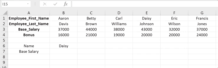
The dataset is the transpose of the dataset used in the vlookup function.

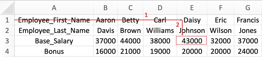
To look up the base salary of Daisy, the hlookup function looks rightwards along the first row until it finds the text “Daisy” (column E).  It then looks downwards across the rows to find and return the value in the “Base_Salary” row.

The hlookup function has the following syntax:

Assume the following dataset [you may paste it to Excel]:

The formula = hlookup(B6, $A$1:$G$4, 3, FALSE) returns base salary of Daisy. Here is the process performed in the hlookup function:

1. 1. What is the lookup key?
      The text “Daisy.”
   2. Where to look up?
      The range A1 through D7.
   3. What to look up?
      The base salary of Daisy, which is in the third row of the range specified in (2).
   4. How to look up?
      An exact match is required.

Multiple-Criteria Lookup

The above lookups are based on a single lookup key (i.e., a single-criterion lookup). While the vlookup and hlookup functions do not deal with multiple lookup keys, the different columns (rows) of the dataset can be joined to create a unique and single lookup key.

Example:

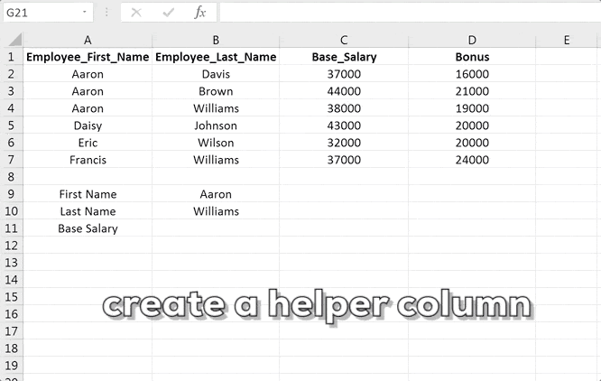
Assume the following dataset [you may paste it to Excel]:

In the above dataset, three employees have the first name “Aaron” and two have the last name “Williams.” To correctly look up the base salary of the employee Aaron Williams, the data in both columns A and B (multiple criteria) must be used. To perform a multiple-criteria lookup using the vlookup or hlookup function, perform the following steps:

1. Insert a helper column (row) to the leftmost (uppermost) of the dataset.
2. Use the concatenate function to join the data in the “Employee_First_Name” and the “Employee_Last_Name” columns (rows) [i.e., = concatenate(B2,C2) in cell A2]
3. Use the combination of the first name “Aaron” and the last name “Williams” as the lookup key. That is, in cell C11, use the formula = vlookup(C9&C10, A1:E7, 4, FALSE) to find the base salary of the employee Aaron Williams.

Limitations of the vlookup and hlookup function

Below are the limitations of the vlookup and hlookup function:

1) The functions only perform single-direction lookups. Consider the following dataset:

The vlookup function only looks up data downwards and rightwards. For example, the formula = vlookup(“Aaron”, A1:D7, 1, FALSE) does not return the base salary of Aaron Davis. Rather, it returns an error. Thus, to use the vlookup and hlookup functions, the lookup key must be located on the leftmost (uppermost) of the dataset.

Also, the two functions cannot search the dataset in reverse order (e.g., bottom-up or from right to left).

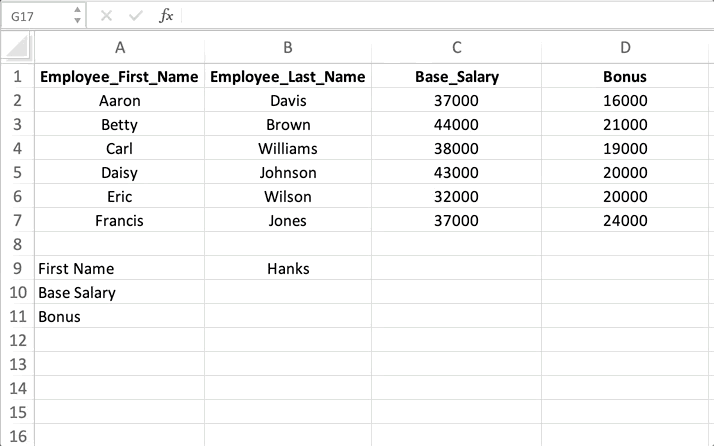
2) The functions return errors when the value is not found. Consider the following dataset:

The formula = vlookup(“Hanks”, A1:D7, 3, FALSE) returns an error because the name “Hanks” is not contained in the list of names.

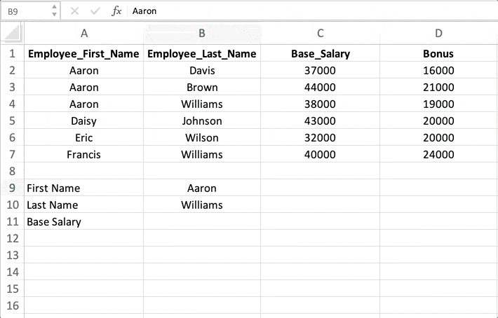
3) An inserted column (row) distorts the result. Consider the following dataset:

If a column named “Employee_ID” is inserted between columns B and C of the dataset, the formula = vlookup(“Aaron”, A1:D7, 4, FALSE), which originally returned Aaron’s bonus, returns his base salary because the column index for bonus has changed to 5.

xlookup function [Available in Office 365 or later versions]

The xlookup function enhances both the vlookup and hlookup functions while using a simpler syntax:

Single-criterion lookup

Example 1:

The xlookup function performs the same function as the vlookup function.

In cell B10, the formula = xlookup(B9, A1:A7, C1:C7) looks up the text “Daisy” in the lookup range A1 through A7 (Employee_First_Name column) and returns the corresponding value in the return range C1 through C7 (Base_Salary column).

In cell B11, the formula = xlookup(B9, A1:A7, D1:D7) looks up the text “Daisy” in the Employee_First_Name column and returns the corresponding value in the Bonus column.

Example 2:

The xlookup function can also replace the hlookup function.

In cell B7, the formula = xlookup(B7, A1:G1, A3:G3) looks up the text “Daisy” in the lookup range A1 through G1 (Employee_First_Name row) and returns the corresponding value in the return range A3 through G3 (Base_Salary row).
In cell B8, the formula = xlookup(B7, A1:G1, A4:G4) looks up the text “Daisy” in Employee_First_Name row and returns the corresponding value in the Bonus row.

Example 3:

The xlookup function is not constrained to data lookup in a single direction [i.e., the lookup key does not need to be located in the leftmost column (uppermost row)].

The formula = xlookup(B9, C1:C7, A1:A7) still returns the base salary of Daisy. Similarly, the formula = xlookup(B9, C1:C7, B1:B7) returns her bonus.

Example 4:

The [ifnotfound] argument of the xlookup function allows us to specify what to return if the lookup key is not found.

In cell B10, the formula = xlookup(B9, A1:A7, C1:C7, “No Records”) specifies that when the lookup key is not found in the dataset, the function returns the text “No Records” instead of an error.

Example 5:

The insertion of a column (row) does not distort the lookup result. If the formula = xlookup(B9, A1:A7, C1:C7) is originally used to find the base salary of Daisy, inserting a column between columns B and C does not distort the lookup result because the formula is automatically updated to = xlookup(B9, A1:A7, D1:D7).

Example 6:

The xlookup function has 4 modes of matching.

The match_mode argument takes the following numbers:

In cell B10, the formula = xlookup(B9, A1:A7, C1:C7, “No Record”, 0) returns the base salary of Daisy.

Example 7:

The xlookup function allows data lookup in the reverse order.

The search_mode argument takes the following numbers:

In cell B10, the formula = xlookup(B9, A1:A7, C1:C7, “No Record”, 0, 1) returns the base salary of Aaron Davis.

In cell B11, the formula = xlookup(B9, A1:A7, D1:D7, “No Record”, 0, -1) returns the bonus of Aaron Jones but not that of Aaron Davis.

Multiple-criteria lookup

The xlookup function does not require a helper column for multiple-criteria lookups.

In cell B11, the formula = xlookup(B9 & B10, A1:A7 & B1:B7, C1:C7) directly finds the lookup key “Aaron Williams” from the lookup range and returns the base salary of the employee with the first name “Aaron” and the last name “Williams.”

Learning Excel Data Analytics with Gleim

At Gleim, we know learning data analytics is vital for future accounting professionals. That is why we are offering this series of data analytics blogs and continually updating all of our review materials for CPA, CMA, and CIA with the necessary information you need to pass your exams!

We’ll continue our weekly blog series. Check back regularly for all exam news and study tips!

Excel Lessons
Excel Basics
Excel Shortcuts
Excel Calculation Rules
Cell References
Excel Functions
Function Basics
Working with Numbers
Working with Datetime Data
Working with Text Data
Logical Testing
Summarizing a group of data
Filtering and Sorting
Lookup Functions
Tables
Pivot Tables