Contact Us : 800.874.5346 International: +1 352.375.0772


Summary statistics of group data generated by functions such as countif, sumifs, and maxifs reduce a group of data to a single value. However, these summary statistics do not directly identify the specific datum meeting the criteria. For example, the countif function can indicate that there are three exceptions meeting the criteria but cannot specifically identify the three exceptions. Filtering and sorting allow us to extract and view the specific data that meet the criteria while hiding those that do not.
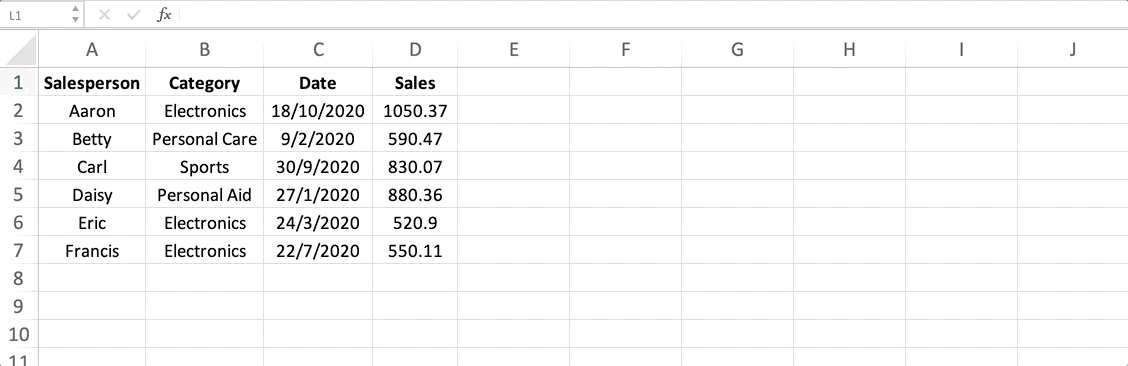
Assume the following dataset [you may paste it to Excel]:
| A | B | C | D | |
|---|---|---|---|---|
| 1 | Salesperson | Category | Date | Sales |
| 2 | Aaron | Electronics | 2020-10-18 | 1050.37 |
| 3 | Betty | Personal Care | 2020-02-09 | 590.47 |
| 4 | Carl | Sports | 2020-09-30 | 830.07 |
| 5 | Daisy | Sports | 2020-01-27 | 880.36 |
| 6 | Eric | Electronics | 2020-03-24 | 520.9 |
| 7 | Francis | Electronics | 2020-07-22 | 550.11 |
Step 1: Select the data to be filtered. (This includes any cell in the dataset.)
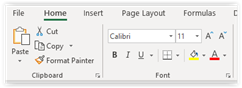
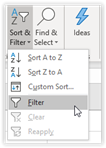
Step 2: Click the following in sequence: Home > Sort and Filter > Filter
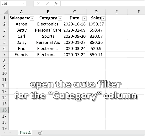
Step 3: Check if there are arrow buttons next to the headers of the columns.

Step 4: To filter a column, click that column’s arrow button to call out the filter. The following is the filter for the “Category” column:
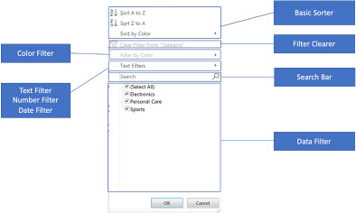
Below are the functions of the different parts of Excel Auto filter:
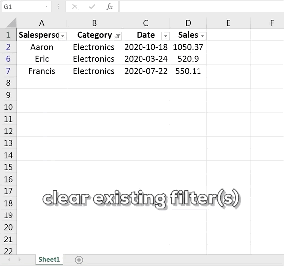
Example: Showing sales only for the “Electronics” category
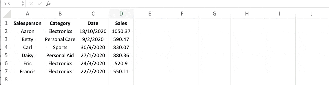
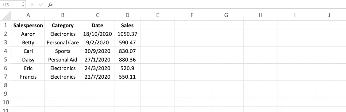
Assume the following dataset [you may paste it to Excel]:
| A | B | C | D | |
|---|---|---|---|---|
| 1 | Salesperson | Category | Date | Sales |
| 2 | Aaron | Electronics | 2020-10-18 | 1050.37 |
| 3 | Betty | Personal Care | 2020-02-09 | 590.47 |
| 4 | Carl | Sports | 2020-09-30 | 830.07 |
| 5 | Daisy | Sports | 2020-01-27 | 880.36 |
| 6 | Eric | Electronics | 2020-03-24 | 520.9 |
| 7 | Francis | Electronics | 2020-07-22 | 550.11 |
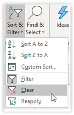
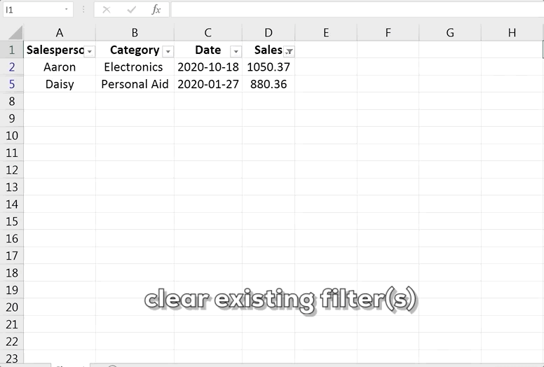
Step 1: Clear any existing filter(s) using the Filter Clearer or the following in sequence:
Step 2: Call the filter in the “Category” column.
Step 3: Uncheck (Select All) in the Data Filter to unselect all the data.
Step 4: Check only the box for “Electronics” to filter out only the “Electronics” category.
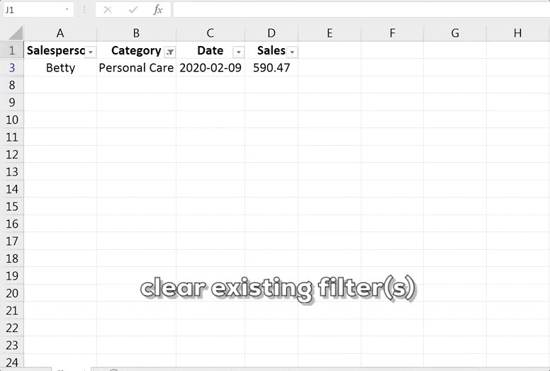
Example: Showing sales only for the “Personal Care” category
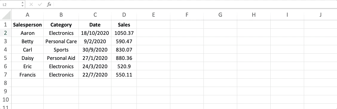
Assume the following dataset [you may paste it to Excel]:
| A | B | C | D | |
|---|---|---|---|---|
| 1 | Salesperson | Category | Date | Sales |
| 2 | Aaron | Electronics | 2020-10-18 | 1050.37 |
| 3 | Betty | Personal Care | 2020-02-09 | 590.47 |
| 4 | Carl | Sports | 2020-09-30 | 830.07 |
| 5 | Daisy | Sports | 2020-01-27 | 880.36 |
| 6 | Eric | Electronics | 2020-03-24 | 520.9 |
| 7 | Francis | Electronics | 2020-07-22 | 550.11 |
Step 1: Clear any existing filter(s).
Step 2: Call the filter in the “Category” column.
Step 3: Type “Personal Care” in the Search Bar.
Example 1: Showing sales between 1/1/2020 and 7/15/2020
Assume the following dataset [you may paste it to Excel]:
| A | B | C | D | |
|---|---|---|---|---|
| 1 | Salesperson | Category | Date | Sales |
| 2 | Aaron | Electronics | 2020-10-18 | 1050.37 |
| 3 | Betty | Personal Care | 2020-02-09 | 590.47 |
| 4 | Carl | Sports | 2020-09-30 | 830.07 |
| 5 | Daisy | Sports | 2020-01-27 | 880.36 |
| 6 | Eric | Electronics | 2020-03-24 | 520.9 |
| 7 | Francis | Electronics | 2020-07-22 | 550.11 |
Step 1: Clear any existing filter(s).
Step 2: Call the filter in the “Date” column.
Step 3: Call out the function list of the Date Filter and choose “Between…”
Step 4: Enter the criteria.
Example 2: Showing sales over $850
Step 1: Clear any existing filter(s).
Step 2: Call the filter in the “Sales” column.
Step 3: Call out the function list of the Number Filter and choose “Greater than…”
Step 4: Enter the criteria.
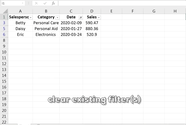
Example 3: Showing sales over $850 in the “Electronics” category.
Step 1: Clear any existing filter(s).
Step 2: Call the filter in the “Category” column.
Step 3: Filter out the “Electronics” category in the Data Filter.
Step 4: Call the filter in the “Sales” column.
Step 5: Call out the function list of the Number Filter and choose “Greater than…”
Step 6: Enter the criteria
The filter function filters a set of data and returns the filtered data based on the specified criteria. It has the following syntax:
![]()
Note: The filter function returns only the data, not the format.
Assume the following dataset [you may paste it to Excel]:
| A | B | C | D | |
|---|---|---|---|---|
| 1 | Salesperson | Category | Date | Sales |
| 2 | Aaron | Electronics | 2020-10-18 | 1050.37 |
| 3 | Betty | Personal Care | 2020-02-09 | 590.47 |
| 4 | Carl | Sports | 2020-09-30 | 830.07 |
| 5 | Daisy | Sports | 2020-01-27 | 880.36 |
| 6 | Eric | Electronics | 2020-03-24 | 520.9 |
| 7 | Francis | Electronics | 2020-07-22 | 550.11 |
Example 1
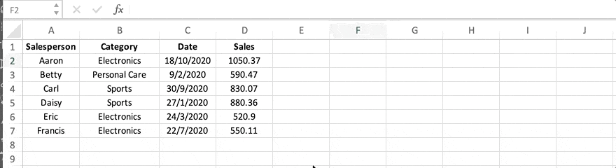
The formula =filter(A2:D7,B2:B7=“Electronics”,“No Records”) looks at the whole dataset from range A2 through D7 and extracts data with the text “Electronics” in the range B2 through B7. If the text “Electronics” is found, the formula returns all the data of the row meeting the criterion. Otherwise, the formula returns the text “No Records.” The sales by Aaron, Eric, and Francis satisfy the criteria.
Note: The range to be filtered should not include the header of each column.
Multi-criteria filter function
Criteria can be added to the filter function using the following operators:
Example 1
The formula =filter(A2:D7,(B2:B7=“Electronics”)*(D2:D7>550),“No Records”) returns the sales that are both in the “Electronics” category AND over $550. If none of the data meet both criteria, the formula returns the text “No Records.” The sales by Aaron and Francis satisfy both criteria.
Example 2
The formula =filter(A2:D7,(B2:B7=“Sports”)+(D2:D7>550),“No Records”) returns the sales that are either in the “Sports” category OR over $550. If none of the data meet either criterion, the formula returns the text “No Records.” All the sales except those by Eric satisfy either criterion.
The unique function filters the unique data in the columns and returns the filtered data. It has the following syntax:
![]()
Note: The filter function returns only the data, not the format.
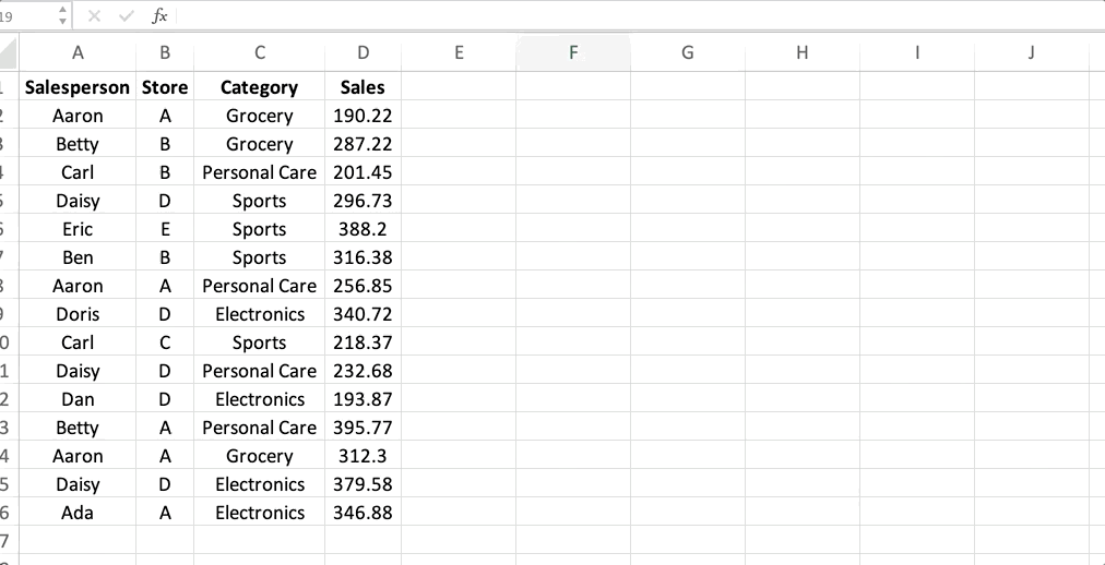
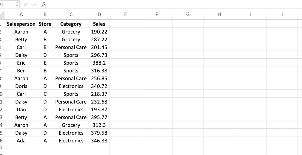
Assume the following dataset [you may paste it to Excel]:
| A | B | C | D | |
|---|---|---|---|---|
| 1 | Salesperson | Store | Category | Sales |
| 2 | Aaron | A | Grocery | 190.22 |
| 3 | Betty | B | Grocery | 287.22 |
| 4 | Carl | B | Personal Care | 201.45 |
| 5 | Daisy | D | Sports | 296.73 |
| 6 | Eric | E | Sports | 388.2 |
| 7 | Ben | B | Sports | 316.38 |
| 8 | Aaron | A | Personal Care | 256.85 |
| 9 | Doris | D | Electronics | 340.72 |
| 10 | Carl | C | Sports | 218.37 |
| 11 | Daisy | D | Personal Care | 232.68 |
| 12 | Dan | D | Electronics | 193.87 |
| 13 | Betty | A | Personal Care | 395.77 |
| 14 | Aaron | A | Grocery | 312.3 |
| 15 | Daisy | D | Electronics | 379.58 |
| 16 | Ada | A | Electronics | 346.88 |
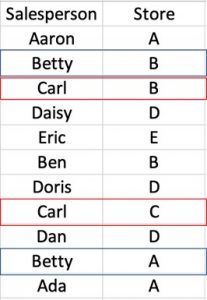
Example 1
The formula =unique(A2:A16) looks at the data in the “Salesperson” column and returns all the unique names of the salespersons.
Example 2
The formula =unique(A2:B16) looks at the data in both the “Salesperson” and “Store” columns and returns all the data that are unique in both columns. For example, in both store A and B, there is a salesperson named “Betty.” The two Bettys are treated as unique because they are from different stores. Similarly, the two Carls, one from store B and the other from store C, are treated as unique.
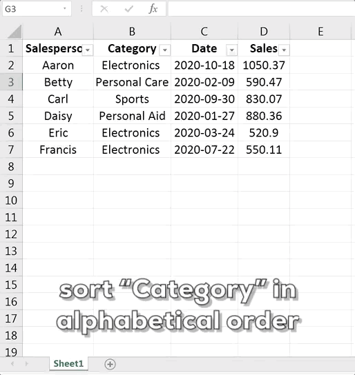
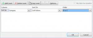
Basic sorting can be done using the Excel Auto Filter.
Assume the following dataset [you may paste it to Excel]:
| A | B | C | D | |
|---|---|---|---|---|
| 1 | Salesperson | Category | Date | Sales |
| 2 | Aaron | Electronics | 2020-10-18 | 1050.37 |
| 3 | Betty | Personal Care | 2020-02-09 | 590.47 |
| 4 | Carl | Sports | 2020-09-30 | 830.07 |
| 5 | Daisy | Sports | 2020-01-27 | 880.36 |
| 6 | Eric | Electronics | 2020-03-24 | 520.9 |
| 7 | Francis | Electronics | 2020-07-22 | 550.11 |
Example 1
The dataset sorted by the “Category” column in ascending order
Example 2
The dataset sorted by the “Date” column in chronological order

Assume the following dataset [you may paste it to Excel]:
| A | B | C | D | |
|---|---|---|---|---|
| 1 | Salesperson | Category | Date | Sales |
| 2 | Aaron | Electronics | 2020-10-18 | 1050.37 |
| 3 | Betty | Personal Care | 2020-02-09 | 590.47 |
| 4 | Carl | Sports | 2020-09-30 | 830.07 |
| 5 | Daisy | Sports | 2020-01-27 | 880.36 |
| 6 | Eric | Electronics | 2020-03-24 | 520.9 |
| 7 | Francis | Electronics | 2020-07-22 | 550.11 |
Multi-level sorting can be done using the following steps:
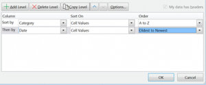
sortby function (available in Officer 365 or later)
The sortby function sorts a set of data and returns the sorted data based on the specified criteria. It has the following syntax:
![]()
Note: The sort_order argument takes the number 1 to indicate sorting by ascending order and the number -1 to indicate sorting by descending order.
Assume the following dataset [you may paste it to Excel]:
| A | B | C | D | |
|---|---|---|---|---|
| 1 | Salesperson | Category | Date | Sales |
| 2 | Aaron | Electronics | 2020-10-18 | 1050.37 |
| 3 | Betty | Personal Care | 2020-02-09 | 590.47 |
| 4 | Carl | Sports | 2020-09-30 | 830.07 |
| 5 | Daisy | Sports | 2020-01-27 | 880.36 |
| 6 | Eric | Electronics | 2020-03-24 | 520.9 |
| 7 | Francis | Electronics | 2020-07-22 | 550.11 |
Example 1:
The formula =sortby(A2:D7,B2:B7,1) takes the whole dataset from range A2 through D7 and sorts it by the range B2 through B7 (the “Category” column) in ascending order.
Example 2:
The formula =sortby(A2:D7,B2:B7,1,D2:D7,-1) takes the whole dataset from range A2 through D7, sorts it by the range B2 through B7 (the “Category” column) in ascending order, and then by the range D2 through D7 (the “Sales” column) in descending order (multi-level sort).
Example 3:
The formula =sortby(A2:A7,B2:B7,1) takes the range A2 through A7 and sorts it by the “Category” column in ascending order. Because only the range A2 through A7 is chosen, the sorted data display only the “Salesperson” column of the dataset and hide other columns.

sort function (available in Officer 365 or later)
The sort function sorts a set of data and returns the sorted data based on the specified criteria. It has the following syntax:
![]()
Note:
The sort function differs from the sortby function in the following ways:
Example 1:
Assume the following dataset [you may paste it to Excel]:
| A | B | C | D | |
|---|---|---|---|---|
| 1 | Salesperson | Category | Date | Sales |
| 2 | Aaron | Electronics | 2020-10-18 | 1050.37 |
| 3 | Betty | Personal Care | 2020-02-09 | 590.47 |
| 4 | Carl | Sports | 2020-09-30 | 830.07 |
| 5 | Daisy | Sports | 2020-01-27 | 880.36 |
| 6 | Eric | Electronics | 2020-03-24 | 520.9 |
| 7 | Francis | Electronics | 2020-07-22 | 550.11 |
The formula =sort(A2:D7,2,1,FALSE) takes the range A2 through D7, sorts it by the 2nd column (“2”, or the “Category” column) in ascending order (“1”) by row (FALSE), and returns the sorted data.
Example 2:
Assume the following dataset [you may paste it to Excel]:
Note: This dataset is the same as in the previous example, transposed (i.e., the columns and rows are swapped).
| A | B | C | D | E | F | G | |
|---|---|---|---|---|---|---|---|
| 1 | Salesperson | Aaron | Betty | Carl | Daisy | Eric | Francis |
| 2 | Category | Electronics | Personal Care | Sports | Sports | Electronics | Electronics |
| 3 | Date | 2020-10-18 | 2020-02-09 | 2020-09-30 | 2020-01-27 | 2020-03-24 | 2020-07-22 |
| 4 | Sales | 1050.37 | 590.47 | 830.07 | 880.36 | 520.9 | 550.11 |
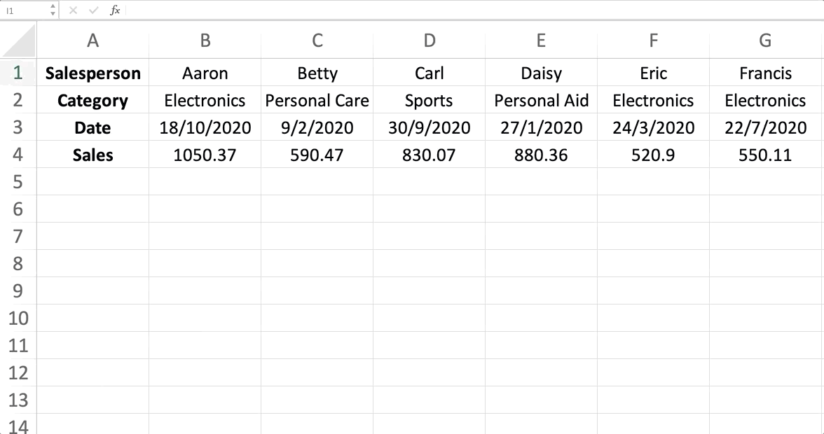
The formula =sort(B1:G4, 4,-1,TRUE) takes the range B1 through G4, sorts it by the 4th row (“4”, or the “Sales” row) in descending order (“-1”) by column (TRUE), and returns the sorted data.
At Gleim, we know learning data analytics is vital for future certified accountants. That is why we are offering this series of data analytics blogs and continually updating all of our review materials for CPA, CMA, and CIA with the necessary information you need to pass your exam the first time!
We’ll continue our weekly blog series. Check back regularly for all exam news and study tips!
Excel Lessons
Excel Basics
Excel Shortcuts
Excel Calculation Rules
Cell References
Excel Functions
Function Basics
Working with Numbers
Working with Datetime Data
Working with Text Data
Logical Testing
Summarizing a group of data
Filtering and Sorting
Lookup Functions
Tables
Pivot Tables
Python Lessons
Python Basics
Conditional Statements
Loops
Functions and Modules
Numerical Python (NumPy)
Pandas Basics
Pandas Data Capture and Cleansing
Merging and Grouping
Manipulating Text and Datetime Data
Visualization
Web Scraping
Errors and Exceptions